Effect of L2 Regularization on Network Weights

02 Sep 2021

Here, we investigate the effect of regularization, specifically weight decay, on the individual layers of a neural network. This post features the same four layer, fully connected neural network featured in a previous post on accuracy and loss congruency. All the code can be found on github.

To start off let’s look at the model’s performance during training. As before, this model is trained on the popular CIFAR10 dataset.

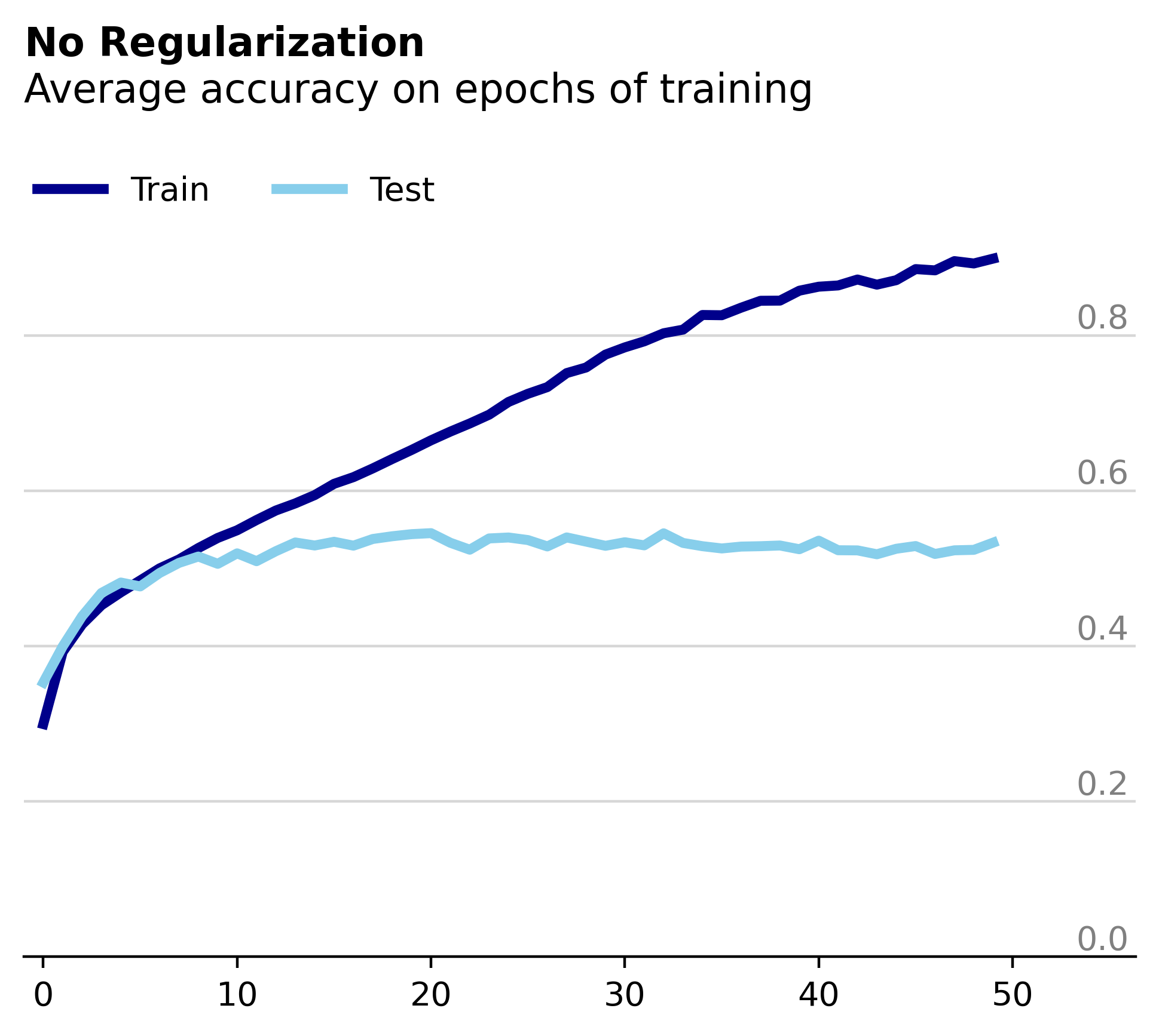
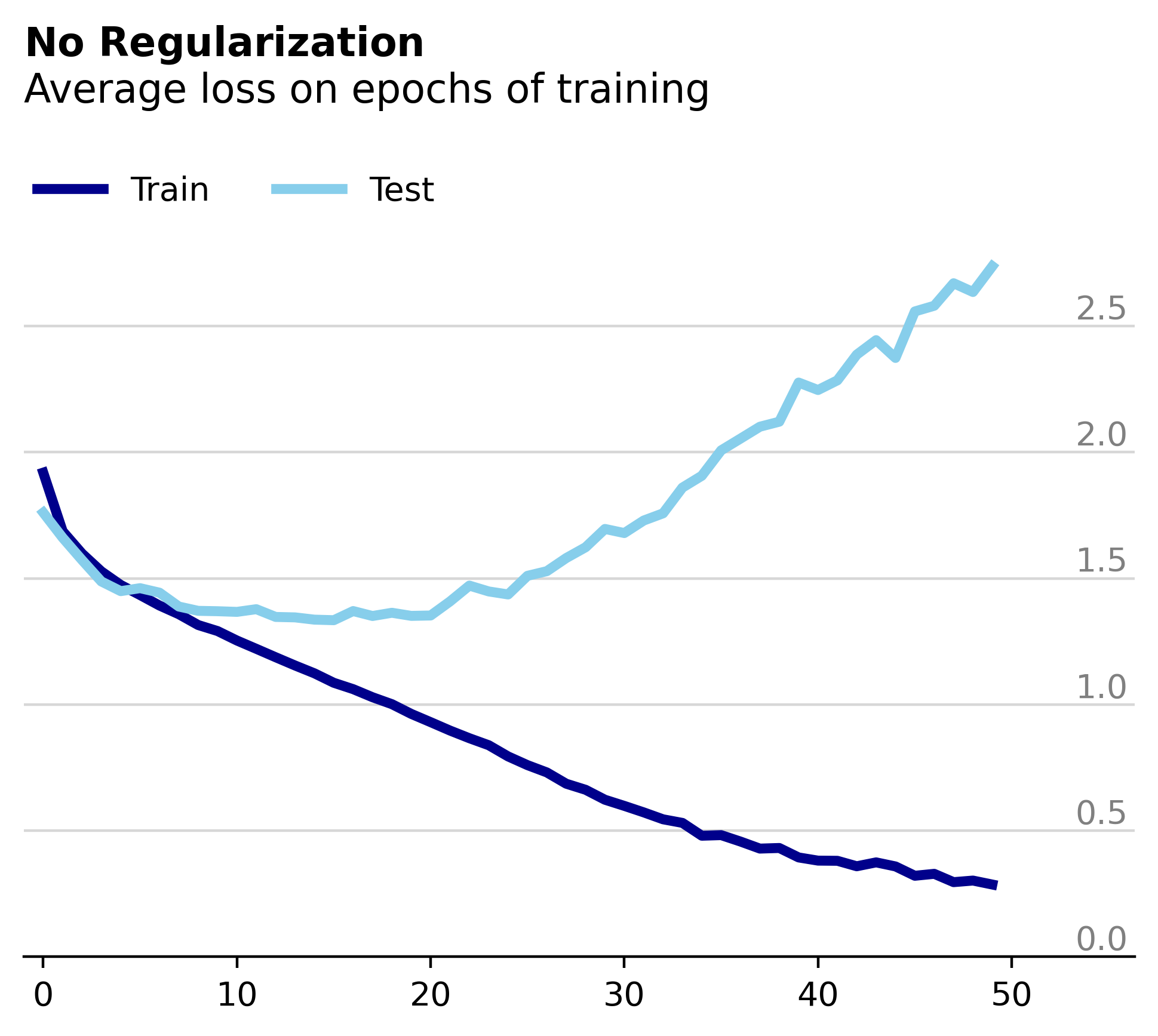
Expectedly, the test and training losses diverge dramatically as the model begins to overfit on the training data. As part of our investigation into the effect of weight decay on the network’s weights we’ll use this unregularized model as a baseline. In this case we’ll compare the percentage of weight parameters in each layer that remain constant between epochs.

Each of the four plots below has an associated tolerance – weight changes within the specified tolerance qualify as “constant”. Formally, let \(w\) be a single weight of the neural network and \(w_{i}\) its value at the \(i\)th epoch. Then if \(|w_{i+1} \: – \: w_{i}| \: \leq w_{i} \cdot tolerance\), we consider the parameter \(w\) to be constant between epochs \(i\) and \(i+1\).

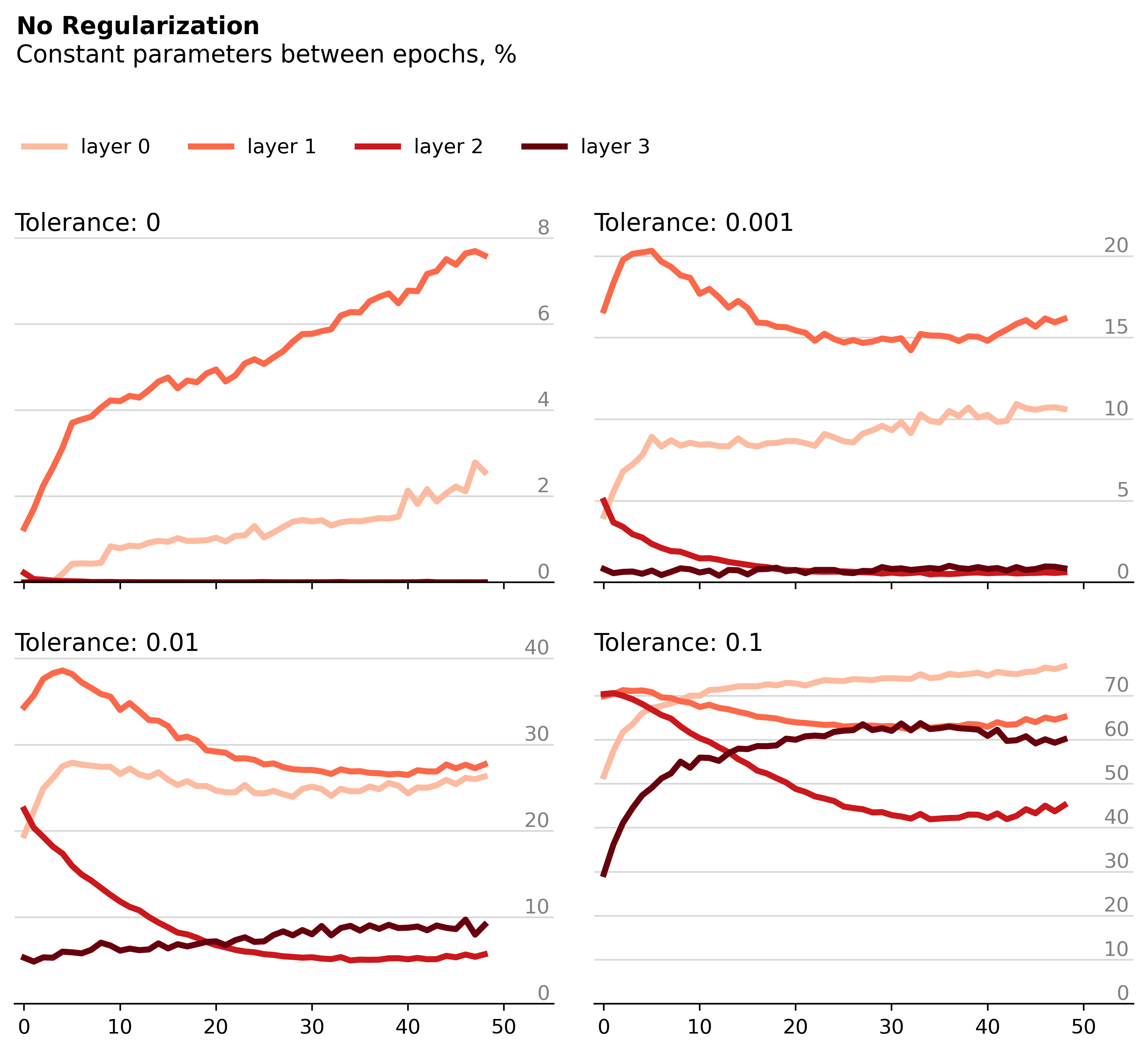
In the upper left-hand plot, we see that a small but significant percentage of the first two layer’s weights remain truly constant between training epochs (tolerance of 0, \(w_{i+1} = w_{i}\)). As we increase the tolerance, we find that ever increasing portions of the network’s layers remain "constant". From the bottom right plot, we can conclude that for most of the network, each individual weight changes no more than 10% between epochs.

Now we train the same model but with added regularization in the form of weight decay.

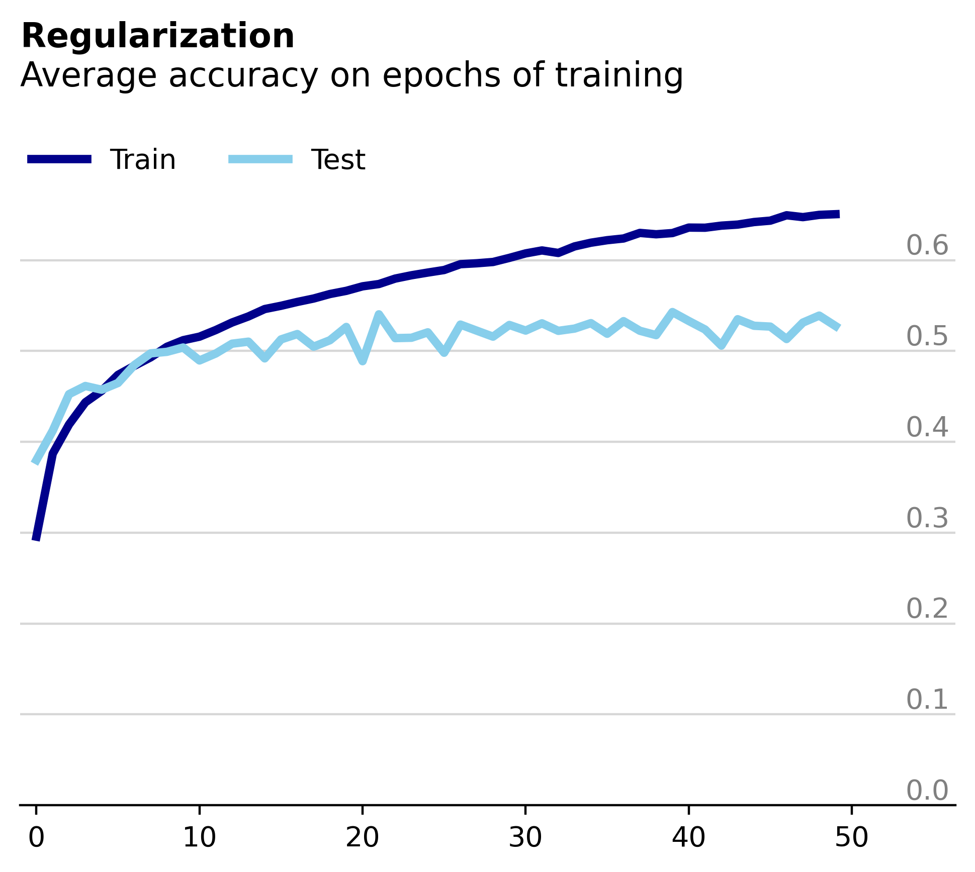
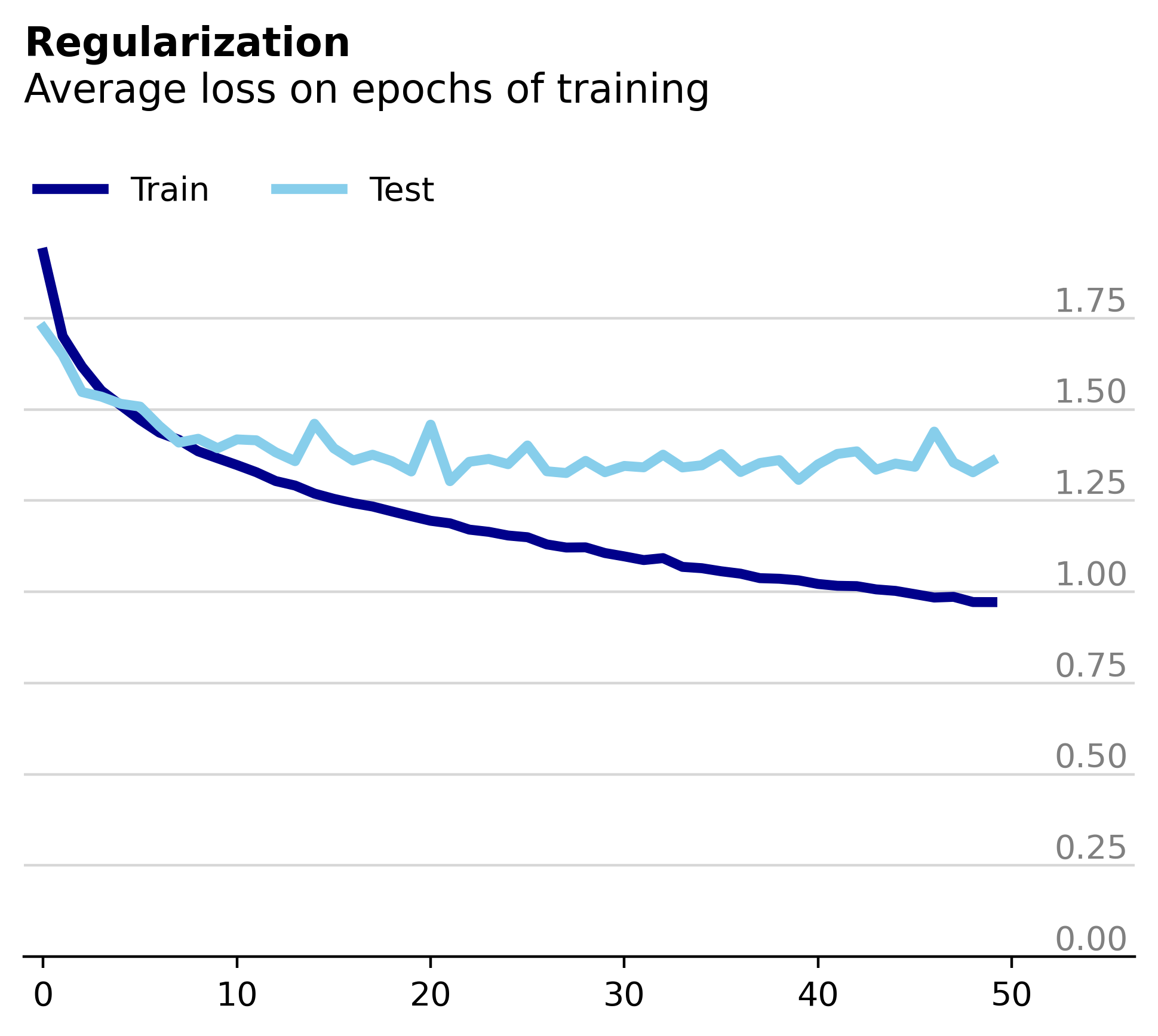
Unsurprisingly, we observe that the train and test loss remain much more comparable, although we haven’t completely solved the overfitting. When we plot the percentage of constant parameters between epochs, we see that the model is much less consistent.

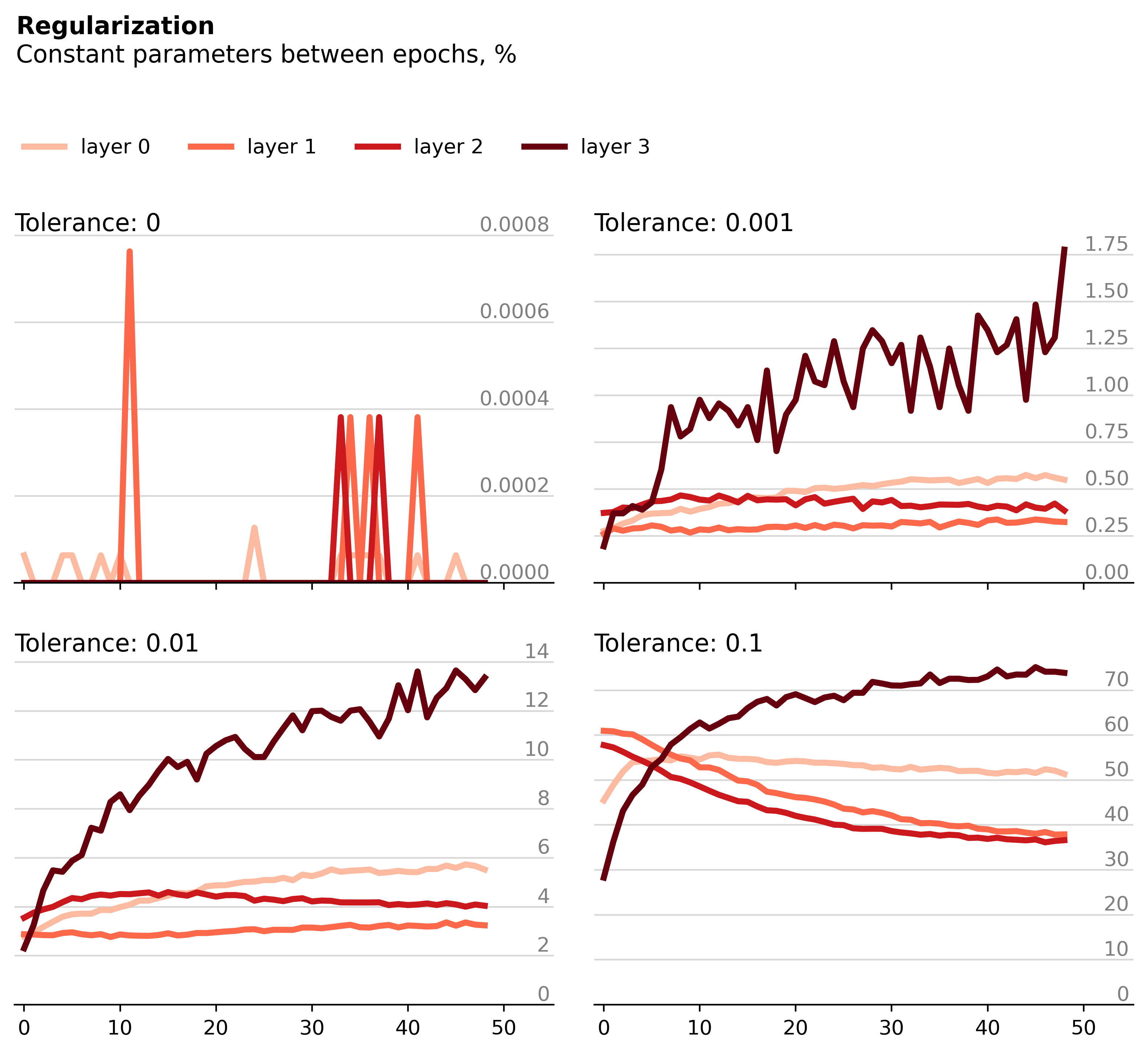
All four layers appear much less stable than the unregularized model, most strikingly at smaller tolerance values. Since L2 regularization works by applying a squared penalty of each weight, larger values are penalized much more than smaller ones. Thus, intuitively it makes sense that the regularized model would favor smaller, more distributed weight changes over larger, more concentrated ones.

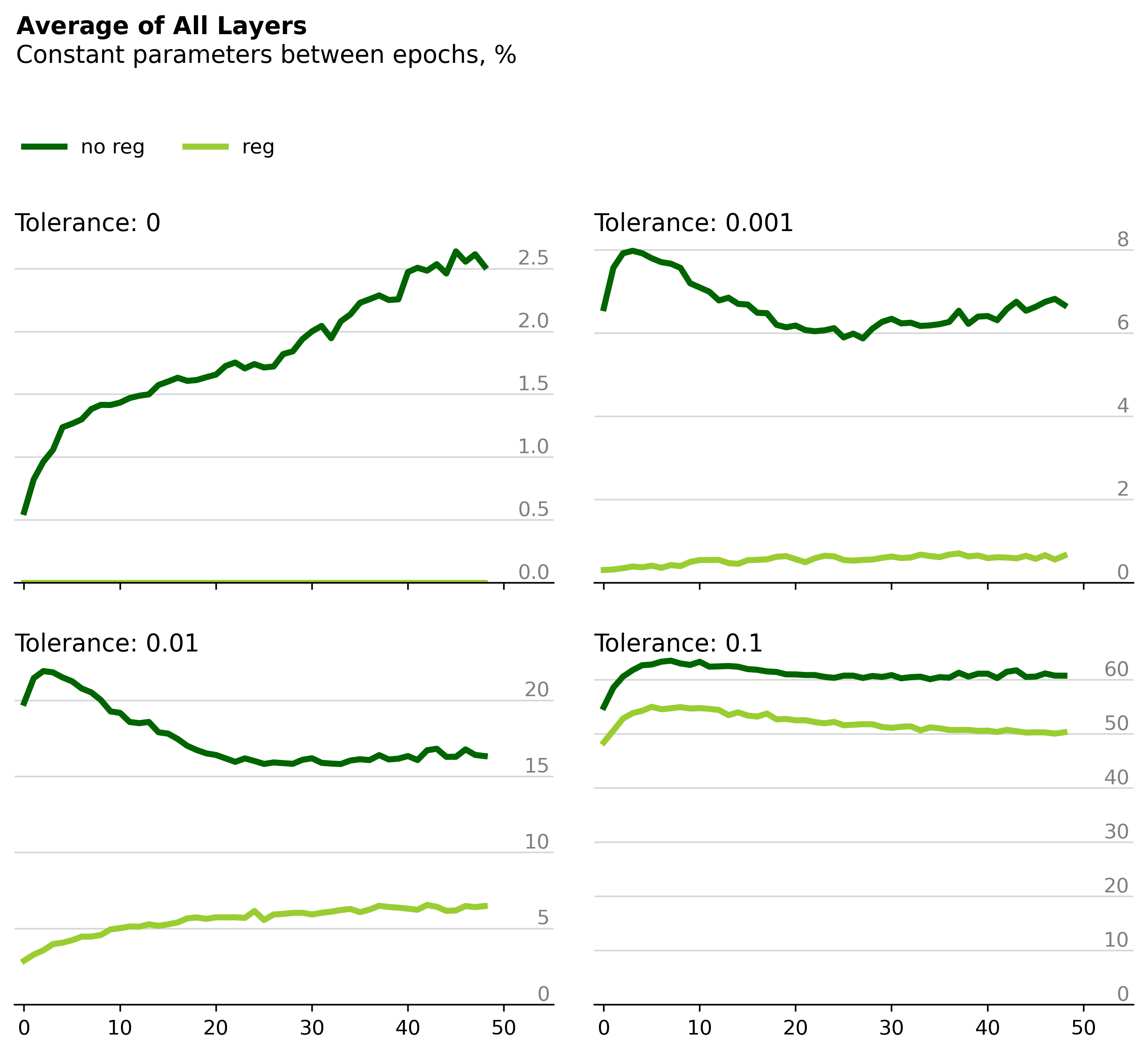
If we average the percentage of constant parameters across all four layers and compare the two networks directly, we can see clearly that regularization appears to decrease the number of constant parameters between epochs.

If we look at the same plot but only average across the last two layers, the regularized and unregularized models appear nearly indistinguishable.

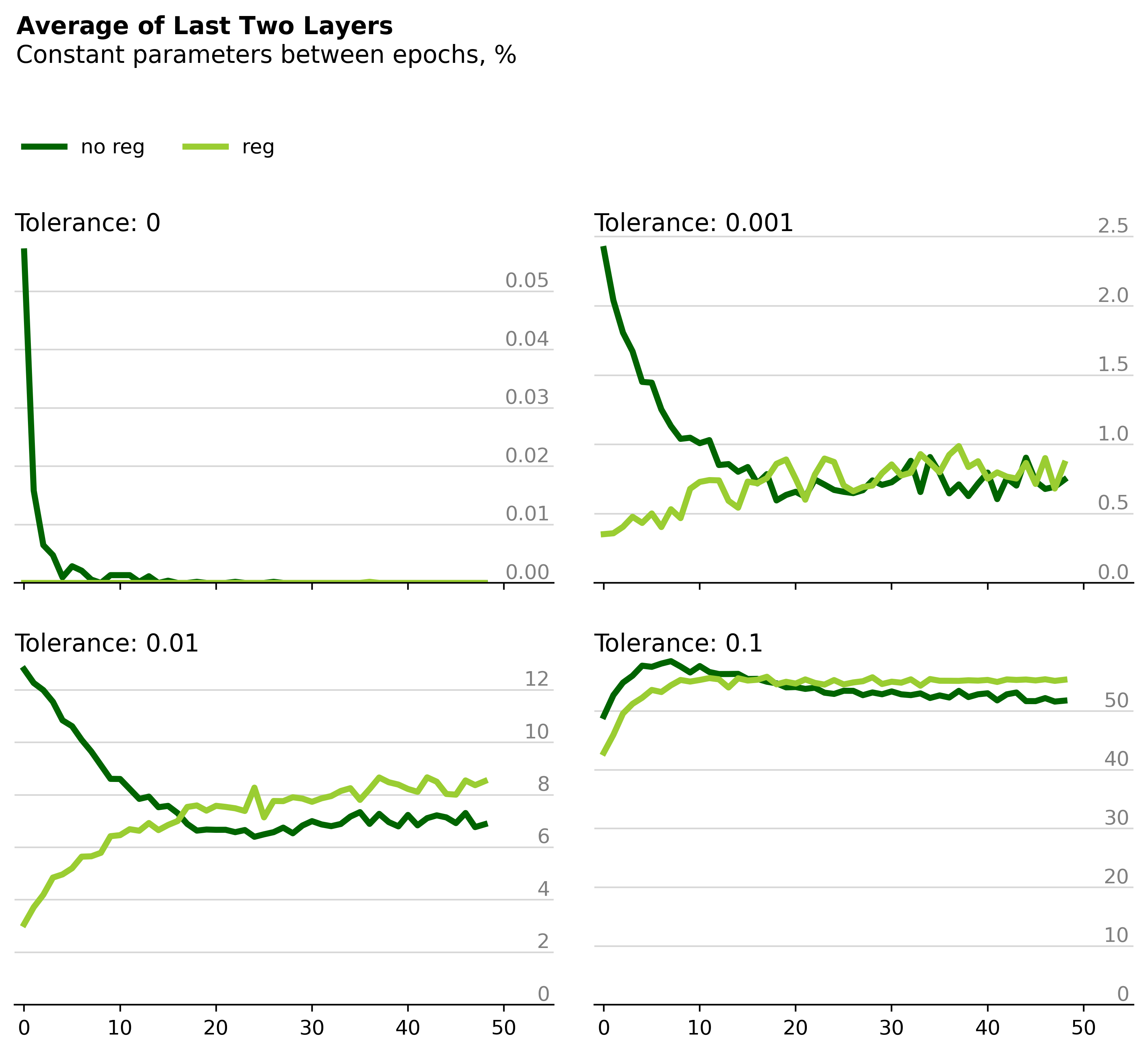
Ultimately, it appears that in this small example regularization causes the network to update more of its parameters from epoch to epoch during training. Conversely, the unregularized model seems to rely on a smaller subset of its weights. This effect is most prominent in the earliest layers of the network, presumably where lower-level features are learned.